-
 RegMult: Multivariate regression and residual interpolation
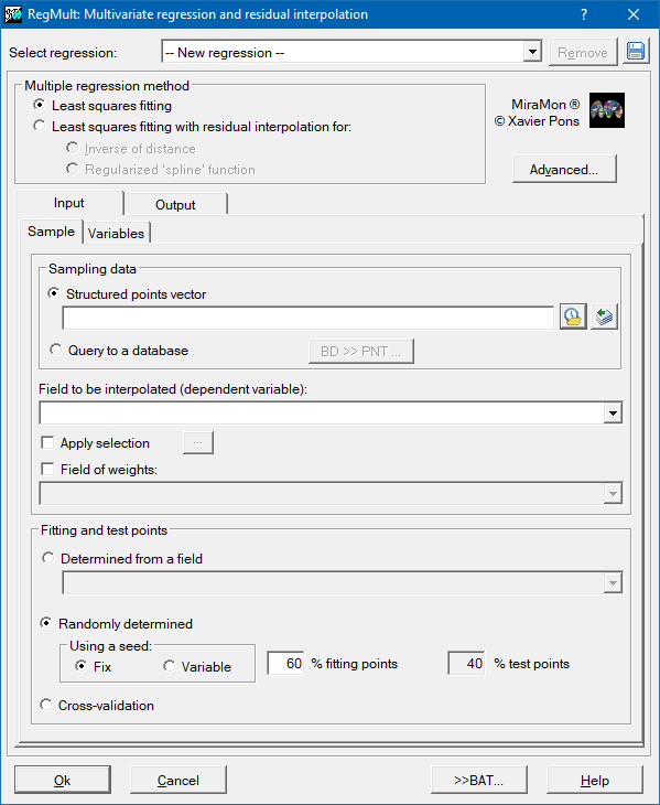
RegMult: Multivariate regression and residual interpolation| Presentation and options | Dialog box of the application |
| Syntax |
The model applies multiple linear regression in such a way that the Y dependent variable is obtained from the xn independent variables, using an expression of the following type:
![]()
The a0, a1,... an coefficients are fitted for least squares. The application offers the possibility of adding a spatial interpolation of the resulting residuals, in such a way that the predictive power is in many cases improved so that the interpolation can account for most of the variance that is not explained by the multiple regression.
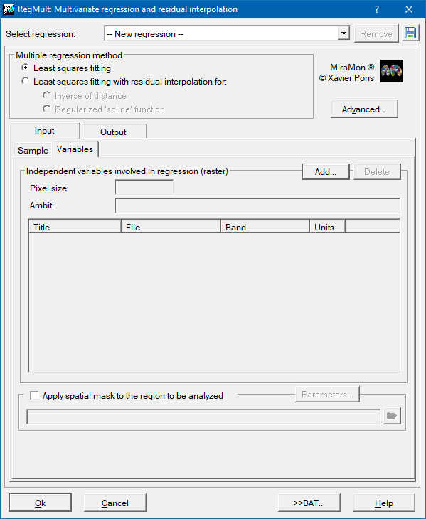
In order to determine the regression coefficients it is necessary to provide a set of samples in which the dependent variable is known in specific (precise) locations and all the possible independent variables. These samples are provided either in a structured PNT point file, or in a DBF format table, or in a table in any of the formats that are accessible with an ODBC driver (Open Database Connectivity). The independent variables should be provided as raster in IMG format of the same geographical area and pixel size. The predictive result will also be a raster in IMG format.
The process to create the resulting raster has two phases (or a single phase in the simplified version of the algorithm): regression and interpolation.
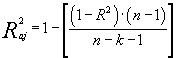
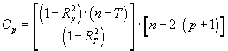
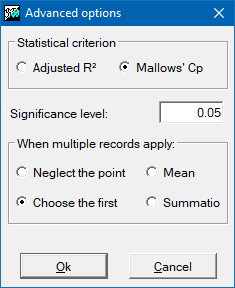
The regression procedure is, in fact, an iterative adjustment process of all the possible regressions: from the regression with all the independent variables initially entered to regressions with a single independent variable. Analyzing the statistical parameters of each regression and, depending on the criterion chosen (best R2 adjusted coefficient or Cp Mallows), the best of all the regressions possible is obtained (provided that the lowest acceptable significance threshold is exceeded).
|
n: number of adjustment points k: number of independent variables R2: coefficient of determination |
p: number of independent variables selected T: maximum number of independent variables n: number of adjustment points |
During the selection procedure for the optimum regression, the application provides information about the statistical parameters of the regression with all the independent variables entered and about the statistical parameters of the regression selected (only if both solutions are different) and in this way it is able to evaluate how the selected regression improves by eliminating any variable which has been detected as having low significance.
If the user has selected only the multivariate regression option, the resulting model will be generated by calculating the solution of the selected regression throughout the area of the study using the adjusted coefficients applied to the independent variables necessarily defined throughout the area of the study.
If the user has chosen to obtain the model with the complete algorithm (regression and residual interpolation), there will be a second phase consisting on the calculation of the residuals of the sample of adjustment points. The residuals are obtained by calculating the differences between the model predicted by the multivariate regression and the known value of the dependent variable. These residuals, known only in the locations of the adjustment points, will spread throughout the area of the study through interpolation. The user will be able to choose between two interpolation methods: Inverse distance weighted (IDW) or regularized spline function. The parameters and the features of the two methodologies can be consulted in InterPNT.htm.
The search for the set of parameters which will produce the optimum interpolation of the residuals is an important step. The results of the interpolation, and of the method as a whole, may vary significantly depending on which set of parameters is applied. Consequently, it is highly advisable to reserve an independent sample of the data points in order to carry out the verification test. This test will mainly consist in calculating the total RMS (root mean square) of the test points, checking that there is no single point with an excessively high error. This (RMS) indicator provides a good base for accepting a given set of parameters. Other complementary criteria could be the assessment of the presence of artifacts in the interpolation, the detection of a systematic error, etc.
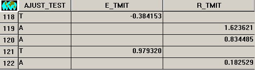
In order to facilitate the analysis, which should provide the best possible model, the application offers the option of generating two resulting layers. The first is a vectorial point layer which contains the valid points with data which, either participate in the adjustment and are later used to interpolate the known residuals, or serve as a test to validate the interpolated solution. For the test points, the user is informed in the database of the residual obtained as the difference between the known value and the predicted value (regression+interpolation), and for the adjustment points, the residual obtained is reported as the difference between the known value and the predicted value (regression only). The following illustration shows these details.
The other resulting layer, which is optional and informative, is the raster resulting from the interpolation of the residuals. An inspection of this layer allows one to carry out an in-depth analysis of the interpolation phase which is separate from the regression. It can be used to analyze if the interpolation has generated unwanted artifacts, too many out of range values, areas with too much variability, etc. It can also be a useful source for getting to know and investigating the areas that display variability which is inadequately registered by the independent variables.
In principle, all the points which have valid data within the area of the study of the PNT file with the samples will be used either as adjustment points or as test points. In addition, the application allows to filter out those data which are not considered appropriate by applying restrictions to the database. If the sample does not have an explicit graphic layer, in which case the fields must necessarily be defined with the coordinates, the restrictions will be applied using an SQL (Structured Query Sentence). Once the whole of the sample to be used has been selected, how it is to be subdivided into adjustment points and test points must be decide.
The choice regarding which points of the sample will be adjustment points and which will be test points can be left as a random option indicating only which proportion (%) will correspond to adjustment points and which proportion to test points. This random choice may originate from a fixed seed (generating reproducible sub-samples, or using a variable seed (obtaining different sub-samples in every new execution). It is also possible to decide by means of a field of a database by assigning the value A to the adjustment points and the value T to the test points. It is also possible do a cross validation. In this case the output raster is obtained using all points as adjustment points and, to do the tests, an iteration process is done, in number equal to the total number of points, where in each one of them the adjustment is made again leaving out one point to carry out the test.The final RMS is calculated as the square root of the average error of each iteration previously squared. This type of validation is specially interesting when the dependent variable has little samples, all samples are essential and it can not dispense with any point in using them as test. Using the cross validation all samples are adjustment and test both.
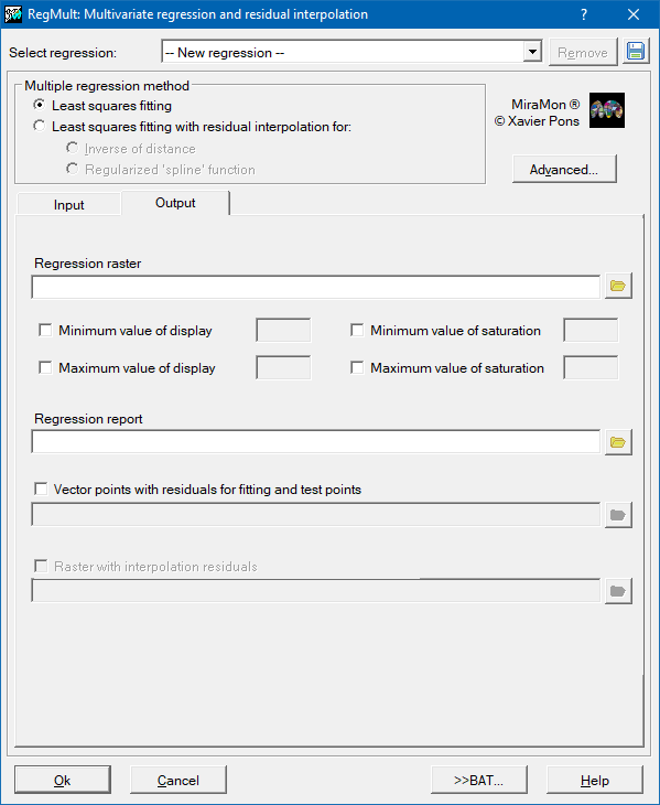
The two obligatory resulting files are a text plain, which contains information about how the whole process has been carried out, and the raster with the predictive model.
The text file gives information about which options the user has chosen, what the adjusted coefficients of the regression are, both those which are used to reproduce the multivariate model and the normalized coefficients (reduced to comparable ranges of mean 0 and deviation 1) in order to be able to analyze the influence of each independent variable on the model, which independent variables have been discarded and what are the main statistics of the selected regression and of the whole. Finally, information is given regarding the quality of the model by means of the RMS of the test points, which is also recorded in the metadata of the resulting layer.
The IMG raster resulting from the predictive model will have the same geographical area and pixel size as the rasters of the independent variables; it is possible to delimit, by means of an exclusion mask, the areas in which it is not necessary to calculate the resulting value (by giving it a NoData tag). By opting not to calculate the solution of the model for these areas, it is possible to considerably accelerate the execution speed. It is also possible to define extreme visualization values (minimum and maximum) which make it possible to produce visually-comparable maps by maintaining the assignation between the range of values and the colors of the assigned palette constant.
More information can be consulted at the following reference:
Ninyerola M, Pons X, Roure JM (2000) A methodological approach of climatological modelling of air temperature and precipitation through GIS techniques. International Journal of Climatology 20: 1823-1841. DOI: 10.1002/1097-0088(20001130)20:14<1823::AID-JOC566>3.0.CO;2-B. https://rmets.onlinelibrary.wiley.com/doi/epdf/10.1002/1097-0088(20001130)20:14<1823::AID-JOC566>3.0.CO;2-B.

 |
| RegMutlt dialog box |