ICT: Compute the Terrestrial Connectivity Index

Access this help text as a web page: ICT

Presentation and options	Dialog box of the application
Syntax

Presentation and options

In the field of ecology, ecological or terrestrial connectivity is defined as the ability shown by the different habitats that form a territory to allow the movement of several organisms through them. Connectivity is calculated through the spatial distribution and the characterization of these habitats. If not having habitat maps, connectivity can also be calculated via land cover or land use maps.

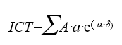
This application generates a raster layer that covers a certain study area, where each cell contains the Terrestrial Connectivity Index (TCI) for that cell center, or focal point, according to Pino formula, modified from that of Hanski.

TCI=Sum_of_the_cell_area_surrounding_the_focal_point

where:

the area (A) of each cell surrounding the focal point is conserved if the affinity (a) with the focal category is 1 and gets smaller the lesser this affinity is. Simultaneously, the area of every surrounding cell also gets smaller the higher the distance between the cell and the focal point is and the higher the impedance is, which is used in the cost distance calculation, δ. A very high impedance makes δ to be high and that cell practically does not contribute to the sum of the connectivity area, whereas a minimum impedance, equaling 1, makes δ to become the Euclidean distance and its contribution to the sum of the area is proportional to the negative exponential of the Euclidean distance; the contribution of the impedance is multiplied by a value α which provides an estimation related with an average dispersion of the species in a minimum impedance situation and which is established on a contribution of 0.05 times the area in a distance equal to the maximum exploration radius: α=-ln(0.05)/radius. In other words, the third factor (exponential function) applications that the contribution of the area is multiplied by 1 when the distance is 0 and the impedance is minimum, that is multiplied by 0.05 when the distance is the maximum exploration radius and the impedance is also the minimum one (1), and that it could be multiplied by practically zero when the impedance is high.

In order to scale appropriately the results, and as justified down below, a base 10 logarithm is finally applied to the result.

The calculation is made for a certain habitat or land cover/use of interest, named focal category, TCIc. As explained later, it is possible to combine TCIc of different categories in order to obtain a general terrestrial connectivity index, TCIg.

Essentially, TCI provides, on each cell of the obtained raster (i.e., on each focal point), an indicator of the available area (connected) to its surroundings (up to a defined maximum radius) for a determined focal category by which that raster has been calculated. In order to calculate the result, the program adds the areas (cells) surrounding every focal point, but weighting them according to their affinity with the focal category (a related category contributes more to the sum) and, at the same time, weighting the area of each cell according to its cost distance to the focal point (applying a higher cost or "friction" than the pure geographic distance according to the impedance of the cell category regarding the focal category).

In order to obtain the Terrestrial Connectivity Index of each focal point and writing it on each cell of the resulting raster, this application determines its connectivity according to a surrounding area based on:

a raster file of impedances

Impedance can be defined as the resistance to connectivity of a category (a habitat or land cover/use) regarding the focal category.

The program uses a raster file that provides, for each cell in the study area (for example, of 30 m side), the impedance with the subject-matter focal category. It is obtained based on a reclassification of the habitats file or land covers/uses file to the adequate impedance values of each category regarding the focal category. The impedance allows considering a non-Euclidian distance between the analyzed points, modified by an anisotropic cost that exists when considering connectivity in a real landscape, made out of different habitats or covers placed in different positions around each focal point.

Impedance is minimum (1) when it is between the focal category and itself or very close categories. Impedance is maximum (for example, 1000, a value that makes connectivity practically impossible) when it is between itself and other categories when considering that connectivity is practically nonexistent (between forests and urban areas, for example).

Impedance is established by experts in the connectivity of each habitat/land cover/use regarding other habitats/land cover/uses. Often, the term impedance is used as the inverse of affinity, described next.

There can be impedance cells tagged with NoData values, which will be excluded from the calculation.

a raster file of affinities

Affinity can be defined as the similarity shown by a category (a habitat or a land cover/use) in accordance with the focal category, and which allows connectivity between both.

The program uses a raster file that provides, for each subject-matter cell (for example, of 30 m side) the affinity with the subject-matter focal category. Affinity is obtained by reclassification of the habitats file or land covers/uses file in the adequate values for each category regarding the focal category.

Affinity is maximum (1) when it is between the focal category and itself, or between itself and very similar categories. Affinity is minimum (for example, 0.001, a value that makes connectivity practically impossible) when it is between itself and other categories when considering that affinity is practically nonexistent (between forests and urban areas, for example).

Affinity is established by experts in the connectivity of each habitat/land cover/use regarding the other habitats/land cover/uses. An approximation is the number of shared organisms between each couple of habitats/covers/uses.

There can be affinity cells tagged with NoData values, which will be excluded from the calculation.

Since impedance and affinity raster files are clipped iteratively, in order to obtain the maximum execution speed, it is preferable that those are, or an uncompressed IMG (maximum clipping speed although this occupies more disk space), or extra-compressed indexed files (indexed RLE files; users can check this in GeM+, or convert uncompressed into indexed RLE files using IMGIMG).

distance between focal points

Users have to define the separation distance between focal points where the calculation of the TCI has to be done. This distance is expressed in the units of the Horizontal Reference System of the original files (of impedances, etc). The raster file of TCI will have the same cell side value as in the defined focal points (or samples) distance.

Often it is not necessary (and it will slow down the process) to apply the calculation to a distance between focal points being equal to the cell side of the original habitat or land cover/use maps, because the calculated connectivities in a cell and its adjacent cell are practically the same. Due to this, the distance between focal points usually is a higher value than the one of the original cells. In addition, the distance between focal points must be a value that, divided by the cell side of the original files, the given result is an odd number (the program controls this and issues an error message if this condition is not met). For example, if working with a raster with cell side of 30 m, distances between focal points of 150 m, 210 m or 390 m can be adequate values; values that are progressively higher will make a quadratically faster execution of the program or of the BAT/PS1 resulting from the program, but the TCI determination will be less precise; this imprecision will be translated into more discontinuities between cells, but above all, into the possible non-observation of areas with a better or worse connectivity due to an excessively separated sampling.

It is recommended to perform some tests in a window of the study area in order to have a successful perception of which distance between focal points is the most suitable one in that area, taking into account its landscape structure and the cell side provided in habitat or land cover/use maps. It must be taken into account that the applied formula on each focal point adds the areas of all the surrounding cells (up to the radius stated next) weighted by the affinity with the focal category and, at the same time, weighted by the cost distance (anisotropic, which considers impedance) of each cell to the focal point. Regarding the influence in the calculation time, users can consult point 1 in advanced issues.

radius of the explored area surrounding each focal point

Users have to define the radius surrounding each focal point by which the calculation will be performed. In practical terms, and in order to accelerate calculations, instead of applying a circular radius, a squared influence area defined by a semi-side will be used. So the radius corresponds to the semi-side of squared subject-matter areas and it must be a value that, when doubled and divided by the cell side of the original files, the given result is an odd number. If working with a cell side of 30 m, 2025 m can be an adequate value; values that are progressively higher will make a quadratically slower execution of the program or of the resulting BAT/PS1, but giving a raising of precision in TCI determination each time smaller, given that exploration in far cells has little weight in the final TCI raster cells obtained. Often this radius is a higher value than the distance between focal points, but is well-tolerated that it could be smaller for exploration purposes, for example, in order to obtain faster preliminary results (given that a value smaller than the exploration radius makes a faster calculation). It should be noted that, since the distance effect decreases exponentially, creating a very big radius will imply much more calculation time and the results will be practically the same. Furthermore, for more information, users can consult point 2 in the advanced issues.

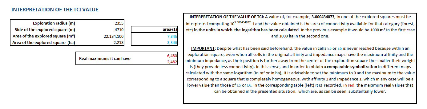
The obtained TCI will be shown in a raster file that expresses on each cell the base 10 logarithm of the connectivity surface of the cell (adding 1 to the surface to avoid negative values of the logarithm). A logarithm is applied in order to have some adequate value ranges in the map (on one hand, the index calculated in this way has smaller values and, at the same time, the bigger and more different values are closer, while it is possible to better distinguish the values of lower and medium connectivities).

This raster file will have a cell side equal to the distance between focal points stated by the user.

The application allows choosing the units of the TCI file, both in hectares (ha) adding 1 to the value because of the previously expressed reasons, and in m² (+1) if desired (an option that could be convenient if working with short distances where the consideration "by m²" could be more natural than the consideration "by ha"). In order to clarify the unit expression, the output file states log(ha) or log(m²), although what is really calculated is log10(ha+1) or log10(m²+1).

As previously said, users typically want to obtain a TCIc for each habitat or land cover/use of interest (forests, crops, etc.), via executions of this program. Later, a general TCI can be obtained by doing an average of the different rasters (TCIc, by TCI of each cover) with the application EstRas (or with CalcImg). This average is an approximation that weighs the different habitats or covers on equal terms: users can consider doing a weighted average according to the proportion of each cover on each cell as a more realistic approximation. Also, users can densify any of these resulting files to the resolution of the original habitats or land cover/uses map; it is suggested to perform it by selecting bilinear interpolation in the DensRas application.

If the value of the index has to be reverted to the connectivity surface value of each cell (in ha or m², according to how it has been calculated), enabling the function POW() of CalcImg application, will directly perform the operation: layer_surface=10^(layer_TCI)-1.

If a structured point layer (.pnt, vector) with the TCI of each focal point excluding the cells that ultimately could located with NoData areas (sea, etc) is desired, users can run the application IMGPNT; please note that if not having the different TCI of the several habitats or covers of the studied area configured as a multi-band raster, IMGPNT allows obtaining the .pnt in a single operation, that will create as many fields in the attribute table of the .pnt file as bands contained in the multi-band raster.

Alternatively, it is possible to state that two additional layers want to be created, one of them with centered points on each focal point and another with polygons delimiting the analyzed area on each focal point. These layers do not directly intervene in the calculation process, but can be useful to have a visual idea of the sampling density and the geographical scope of each point, something useful when teaching, for example. These files will have the same name as the generated TCIc raster, but adding the suffixes "_Samples" and "_Zones", respectively. The attributes of the points and polygons will appear from 1 to the number of analyzed focal points (or samples). These files will be non-structured vectors (.vec); if the number of focal points is very high, its drawing, consult, etc, will be slow, so it could be convenient to convert them into structured files (.pnt and .pol) via the applications VECPNT and Ciclar of MiraMon setting (important!) that topological structuring is NOT desired.

In extensive areas (thousands of km²) with short sampling distances (hundreds of meters) and long exploration radius (kilometers), the execution time can require several hours, or days. That is why the application allows (with the parameters InitRow, FinRow and StripNum) preparing different output raster files or different BAT/PS1 output files in order to parallelize the execution in different computers or in computers with different cores.

Advanced issues

1. Effect of sampling distance in calculation time. If you have chosen to generate the TCI from a BAT/PSA file, the application generated a BAT/PS1 file that, when running it, generates the raster with the TCI index corresponding to each square where the ambit of affinity and impedance area maps provided to the program are sampled. Since the calculation of this application is very intense and can require from hours to days according to the ambit, the sampling distance and the exploration radius, it is noted that once an execution is performed on a certain sampling area (for example 390 m in a study area where users have affinity and impedance maps at 30 m) and the required time is known (for example 1.5 h), in order to approximate the required time if the sampling distance is made in a more detailed way (for example, 150 m), the formula to apply is:

new_time=reference_time*(dist_reference_time/new_dist)²

For example, in the preceding case, the new time will be 1.5*(390/150)²=10.14 h. Note that although the resolution improvement relationship in cell side terms is "only" 2.6 times, time is multiplied by 6.76 (the square of the relationship between the sides).

2. Interpretation of TCI value and symbolization aspects of the result. The following calculation provides complementary information regarding the interpretation of values and their cartographic symbolization.

Dialog box of the application

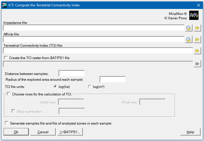ICT dialog box

Syntax:

ICT BATFile Distance Radius ImpedFile AfinFile InitRow FinRow StripNum TCIFile [/UNITS_M2] [/CREA_AUX]

Parameters:

BATFile (BAT/PS1 file that allows TCI raster to be created - Input parameter): NUL or BAT/PS1 file that allows TCI raster to be created. If NUL is given (recommended option) the TCI raster will be generated directly, otherwise a BAT/PS1 file will be generated with a set of calls to various applications that will allow the TCI file to be generated (slower option) .
Distance (Separation distance between focal points - Input parameter): Separation distance between samples or focal points used for TCI calculation; this distance is expressed in the Horizontal Reference System units of the original files (impedances, etc.).
Radius (Radius of the area explored around each focal point - Input parameter): Radius of the area explored around each sample or focal point; this value is expressed in the same units as Distance.
ImpedFile (Impedance file - Input parameter): Impedance raster file name.
AfinFile (Affinity file - Input parameter): Affinity raster file name.
InitRow (Initial row - Input parameter): Initial row (included) of affinity and impedance rasters in which it is desired the TCI calculation to be prepared, numbered from 0 (top row). If the whole raster is desired to be done, enter -1 and -1. Making the program generate the BAT/PS1 so that the calculation is done only in one band (the one defined between the initial and final row) of the raster is practical when you want to parallelize the process to speed it up, starting the BAT/PS1 of each track in a different order session and / or on a different computer. In the end, all you need to do is join all the tiles together with the Mosaic application.
FinRow (Final row - Input parameter): Final row (included) of affinity and impedance rasters in which it is desired the TCI calculation to be prepared, numbered from 0 (top row). If the whole raster is desired to be done, enter -1 and -1. Making the program generate the BAT/PS1 so that the calculation is done only in one band (the one defined between the initial and final row) of the raster is practical when you want to parallelize the process to speed it up, starting the BAT/PS1 of each track in a different order session and / or on a different computer. In the end, all you need to do is join all the tiles together with the Mosaic application.
StripNum (Strip numerator - Input parameter): Strip numerator that will be added to the output TCI raster file name and to the generated BAT/PS1 file name, if this option has been chosen (it is suggested adding 1, 2, etc. to each run). This parameter is not used when InitRow and FinRow are -1, so it is possible to put any value in it (it is suggested 0, which implies that the final file will not have the numerator "_0" pasted into its name).
TCIFile (Output file of the Terrestrial Connectivity Index - Input parameter): Desired name for the TCI raster file. The name of this file does not need to indicate the value of StripNum as the program is responsible for setting it automatically.

Modifiers:

UNITS_M2

CREA_AUX